Neural Image Compression-An Overview

Using neural network to compress image? This is how.

Introduction

Today, I will explore the autoencoder architecture used for neural image compression. Our primary focus is to illustrate how a neural network can be trained end-to-end to achieve balance between image compression efficiency and reconstruction fidelity. Additionally, I will delve into the fundamental concept behind the design of various entropy models.

The Compression Pipeline

Let’s take a brief overview of how image comperssion is generally achieved. Using JPEG compression as an example, the process consists of three main parts: transformation, quantization, and entropy coding. Conversely, the decompression steps are typically the reverse of the compression steps.

Compression

The above animation illustrates the compression pipeline. Initially, the original image (x) undergoes conversion into a latent representation (y) through an analysis transform (g_a in the picture, serving as the encoder part of the autoencoder). Following this transformation, quantization (Q) discretizes each element of the latent image representation, resulting in an integer-valued latent representation. It is crucial to note that this is not the final compressed file; the quantized latent representation undergoes lossless entropy coding (e.g., arithmetic encoding, represented as e_c in the illustration) to generate the ultimate compressed file.

The entropy model offers probability predictions for each element of y hat, playing a crucial role in the entropy coding process.

Decompress

To decompress the compressed file and retrieve the image for display, an entropy decoder (e_d) in the picture decodes the compressed file to get the quantized latent representation back. Subsequently, a synthesis transform (g_s, functioning as the decoder part of an autoencoder) transforms the quantized latent representation back to image space, resulting in the reconstructed image denoted as x hat.

Training Objective

Which parts are learned?

Three models must be trained to implement this data compression pipeline: the analysis transform, the synthesis transform and the entropy model. The primary role of entropy model is to predict the probability of each element in the latent representation.

Rate-Distortion Optimization

Two main goals lie at the heart of any compression task: the bit-rate (efficiency of coding, which can be thought of as the compressed file size) and the fidelity (reconstructed quality of the decompressed image). However, there is an inherent tradeoff between these two goals. If we would like to achieve a smaller file size, the quaility will drop due to a limited bit budget for representing data. Conversely, if we try to achieve high quality reconstructed image, file size will increase to capture a more accurate details. It would be perfect if we could find a method to optimize these two goals simultaneously, achieving an optimal balance. In deep learning, this objective is our loss function, which serves as a lighthouse, guiding the model to learn and achieve our desired objective.

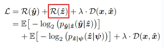
We can write our loss function as follows:

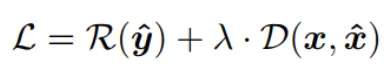
The rate loss term is calculated through Shannon entropy with each probability given by the entropy model. The reconstructed loss term is calcuated through MSE or other perceptual loss metrics. If we can train the entire pipeline end-to-end (as opposed to training each component individually and then combining them), we can expect a compressor closer to the theoritical tradeoff between rate and distortion.

But it’s not such an easy task, because quantization is not differentiable, so the entropy model is a discrete probability mass function (pmf). During training, the derivative of loss function with respect to the parameters of networks g_a, g_s, and the entropy model must be differentiable to allow for back-propagation. The following paragraph discuss how researchers tackle this problem to achieve end-to-end training.

Training End-to-End

Additive Uniform Noise

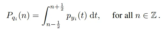
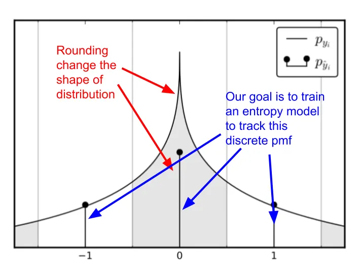
Let’s assume that after an image undergoes the analysis transform, the continuous latent representation follows a Laplace distribution. The actual rounding operation converts this continuous distribution into a discrete pmf, with the probability at each integer value equaling the integration of continous Laplace distribution from -1/2 to 1/2 (which is the bin size of the rounding operation). Our goal is to train an entropy model capable of predicting the probability of each element of quantized latent representation (which is an integer value).

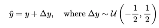
Ballé, Laparra, and Simoncelli in their paper ‘End-to-end optimized image compression’ (2016) proposes a method to overcome the non-differentiability issue of rounding. During training, we add uniform noise, sampled from -1/2 to 1/2, to mimic the rounding operation. This is because rounding from 0.3 to 0 is akin to subtracting 0.3, and rounding from 0.8 to 1 is like adding 0.2. This operation ensures that the decoder will learn to reconstruct data from the degraded latent representation that occurs during inference. Note that we still perform the actual rounding operation during inference once the compressor has been trained and put to work. We only mimic the effect of rounding by adding noise during training, which is a differentiable operation.

Does the additive noise change the shape of the distribtution?

One might worry that the added uniform noise could change the distribution of the quantized latent representation and thus affect the probability estimation. However, we can show that the probability at integer value remains the same.

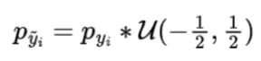
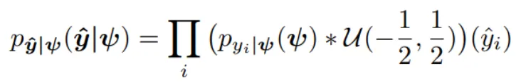
We can write the probability distribution of y tilda as the convolution of y and delta y as follows because the added uniform noise and latent representation are independent.

We can expand the convolution using definition of convolution of two distribution. Note that uniform distribution output 1 in -1/2 to 1/2 and output 0 otherwise.

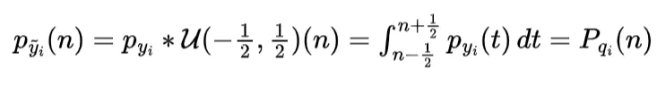
The relaxed continous distribution (p_y tilda) is equal to the original discrete pmf we want to keep track of at integer value.

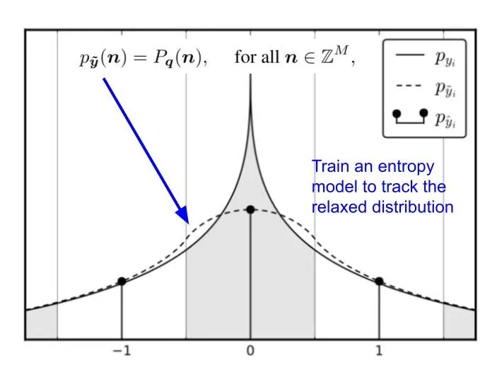
From the graph, we see that the continous latent presentation, after adding uniform noise, is a continous relaxation of the discrete pmf. This suggests that we can use an entropy model to track these relaxed distribution. And once we want to use it for entropy coding, we simply evaluate the continous distribution at the integer values, giving us the probability mass function necessary to construct the arithmetic coding table.

Entropy Model

Factorized Entropy Model

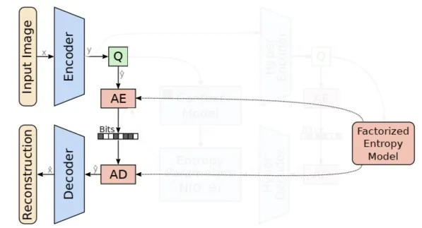
The first entropy model I would like to introduce is the factorized entropy model. In this model, the probability of each element in the quantized latent representation is determined by a separate distribution. The parameters of these distributions are leaned during training. The original paper states that each element is estimated using a non-parametric distribution. This means that the model does not assume a specific distributution shape for the latent representation (note that “non-parametric” in this context does not mean there are no parameters; rather, it means the model doesn’t assume a predefined distribution shape). However, for simplicity, let’s assume that each element is modeled by a Gaussian distribution with mean of 0 and scale of sigma. We then use this Gaussian distribution to predict the probability of each element, outputting a probability value for each one.

The following animation demonstrate the idea, each psi determines the shape of Gaussian distribution, and each element in latent representation A is evaluate through the distribution to get a probability value for entropy coding.

The following code is a toy example of fully-factorized entropy model in pytorch. It is used to estimate the probability of a quantized latent representation tensor in shape [1, 64, 8, 8], where 1 is the batch size, 64 is the channels, 8 is the height and width of the latent representation. The entropy model predict each element using a unique Gaussian distribution with mean = 0 and scale is a learned parameters. By learning **log_scales** instead of scales, you ensure that the exponentiation (**torch.exp(log_scales)**) always results in positive values, thus inherently enforcing the constraint that scale must be positive.

import torch
import torch.nn as nn
import torch.nn.functional as F
class FullyFactorizedEntropyModel(nn.Module):
    def __init__(self, num_channels, height, width):
        super(FullyFactorizedEntropyModel, self).__init__()
        # Initialize the scale parameters for each element in the latent representation
        self.log_scales = nn.Parameter(torch.zeros(1, num_channels, height, width))
    def forward(self, x):
        # Calculate the scales from log_scales to ensure they are positive
        scales = torch.exp(self.log_scales)
        # Assuming a Gaussian distribution with mean = 0 for each element
        # Calculate the probability density function of the Gaussian
        probs = torch.exp(-0.5 * (x / scales) ** 2) / (scales * torch.sqrt(torch.tensor(2 * torch.pi)))
        return probs
# Instantiate the model
num_channels = 64
height = 8
width = 8
model = FullyFactorizedEntropyModel(num_channels, height, width)
# Generate or obtain your quantized latent representation tensor
# For demonstration, let's create a dummy tensor
latent_tensor = torch.randn(1, 64, 8, 8)  # Replace this with your actual tensor
# Calculate the probability of each element in the tensor
probabilities = model(latent_tensor)

The obvious problem is that if I have two different images that, after undergoing the analysis transform and quantization, yield two different latent representation, A and B. In such scenario, our entropy model will predict each element in the same dimension using the same Gaussian distribution with identical parameter. Consequently, this entropy model does not adapt to the specific characteristics of individual images and is not image-dependent.

Hyperprior Entropy Model

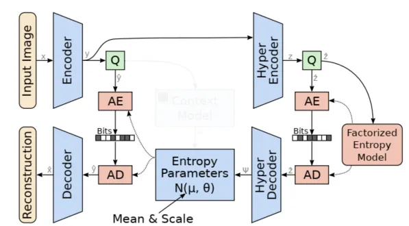
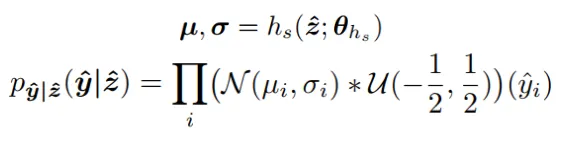
The core idea behind the hyperprior entropy model is to achieve a more acccurate probability estimation for the elements in the latent representation by conditioning on additional side information. This side information aims to capture the global dependencies that remain in the latent representation. To accomplish this, we construct a hyper-network on top of factorized entropy model. This network includes a hyper-analysis network, which transforms latent representation into hyper-latent z. Following this, the hyper-synthesis network is used to estimate the mean and sigma (or sigma only) for each element of latent representation ‘y’.

Image-dependent

This method allows for an image-dependent probability distribution. Each latent representation is first transformed to a hyper-latent, and then a new set of parameters (mean and scale), determined by this hyper-latent, is used for probability estimation.

The following code is a toy example of hyperprior entropy model in pytorch. It is used to output mean and scale for each element of a quantized latent representation tensor in shape [1, 64, 8, 8], where 1 is the batch size, 64 is the channels, 8 is the height and width of the latent representation. The entropy model predict each element using a unique Gaussian distribution with mean and scale as learned parameters.

import torch
import torch.nn as nn
import torch.nn.functional as F
class HyperpriorEntropyModel(nn.Module):
    def __init__(self, input_channels, hyperlatent_channels):
        super(HyperpriorEntropyModel, self).__init__()
        # Hyper-analysis network
        self.encoder = nn.Sequential(
            nn.Conv2d(input_channels, hyperlatent_channels, kernel_size=3, stride=1, padding=1),
            nn.ReLU(),
            nn.Conv2d(hyperlatent_channels, hyperlatent_channels, kernel_size=3, stride=2, padding=1),
            nn.ReLU()
        )
        # Hyper-synthesis network
        self.decoder = nn.Sequential(
            nn.ConvTranspose2d(hyperlatent_channels, hyperlatent_channels, kernel_size=4, stride=2, padding=1),
            nn.ReLU(),
            nn.Conv2d(hyperlatent_channels, input_channels * 2, kernel_size=3, stride=1, padding=1)
        )
    def forward(self, x):
        hyperlatent = self.encoder(x)
        params = self.decoder(hyperlatent)
        mean, log_scale = params.chunk(2, dim=1)  # Split into mean and log scale
        scale = torch.exp(log_scale)  # Convert log scale to scale
        return mean, scale
# Instantiate the model
input_channels = 64
hyperlatent_channels = 32 
model = HyperpriorEntropyModel(input_channels, hyperlatent_channels)
# Generate or obtain your quantized latent representation tensor
latent_tensor = torch.randn(1, 64, 8, 8)  # Example tensor
# Calculate the mean and scale for each element in the tensor
mean, scale = model(latent_tensor)

It’s important to note that the hyperlatent representations must be included in the compressed bitstream alongside the primary compressed image data. During the decompression process, the hyperprior’s decoder utilizes these stored hyperlatent representations to reconstruct the mean and scale parameters of the Gaussian distributions for each element in the quantized latent representation.

Since we do not make any assumptions about the distribution of the hyper-latents, a non-parametric, fully factorized density model is used.

The loss function need to add into a term to account for the bit rate of hyper latent representation.

Context Entropy Model

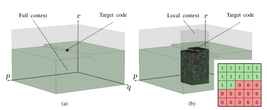
Hyper-prior models capture broader image features, while context entropy model looks at the already decoded neighboring pixels (the causal context) and predicts the distribution of the next pixel based on that context.

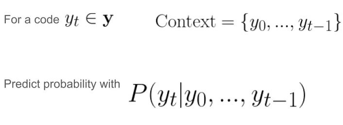
Autoregressive models aims to capture the local dependencies within an image, such as edges or textures, that are immediately adjacent to the current latent variable being predicted. To encode a element y_t, we can utilize y_0, y_1, …, y_{t-1} (previous context). The advantage of this method is that it is bit-free because it directly uses previous elements to estimate the probability of the next symbol. There is no need to store this information in the compressed file. However, the drawback of this approach is its limited efficiency as the operations are inherently serial and cannot be parallelized.

Local content is constrained using a masked convolution layer. The context model (capturing local information) and hyper-net (capturing global information) work together to yield a more accurate estimation of elements in the latent representation.

Conclusion

In this article, we’ve covered the basic learned image compression pipeline. We’ve discussed how the entire pipeline is trained end-to-end and explored the primary types of entropy models used for probability estimation. If you encounter any issues or would like to share additional information, please don’t hesitate to contact me. Cheers!

References

Ballé, Johannes, Valero Laparra, and Eero P. Simoncelli. “End-to-end optimized image compression.” arXiv preprint arXiv:1611.01704 (2016).

Ballé, Johannes, et al. “Variational image compression with a scale hyperprior.” arXiv preprint arXiv:1802.01436 (2018).

Minnen, David, Johannes Ballé, and George D. Toderici. “Joint autoregressive and hierarchical priors for learned image compression.” Advances in neural information processing systems 31 (2018).

Li, M., Zhang, K., Li, J., Zuo, W., Timofte, R., & Zhang, D. (2021). Learning context-based nonlocal entropy modeling for image compression. IEEE Transactions on Neural Networks and Learning Systems.

Liu, Kang, et al. “Manipulation Attacks on Learned Image Compression.” IEEE Transactions on Artificial Intelligence (2023).Ballé, Johannes, Valero